概率分布练习

学习概率分布的基本思路是先明确这个分布有什么用，接着如何去检验，然后如何计算概率，最后在Python里实现。Pyhton实现的步骤是先定义随机变量，之后计算概率，最后用可视化展现出来。

1 离散概率分布-伯努利分布

**import**`` numpy ``**as**`` np ``**import**`` matplotlib.pyplot ``**as**`` plt ``**from**`` scipy ``**import**`` stats ``*# 1 定义随机变量：1次抛硬币。正面朝上为1，反面朝上为0*``X``**=**``np``**.**``arange(0,2,1) X array([0, 1]) ``*# 2 求对应分布的概率：概率质量函数 PMF*``p``**=**``0.5 pList``**=**``stats``**.**``bernoulli``**.**``pmf(X,p) pList array([ 0.5, 0.5]) ``*# 3 绘图*``plt``**.**``plot(X,pList,marker``**=**``'o',linestyle``**=**``'None') plt``**.**``vlines(X,0,pList) plt``**.**``xlabel('随机变量，：抛硬币1次') plt``**.**``ylabel('概率') plt``**.**``title('伯努利分布：p=0.5') plt``**.**``show()

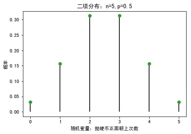
2 二项分布

*# 1 定义随机变量：5次抛硬币，正面朝上的次数*``n``**=**``5 p``**=**``0.5 X``**=**``np``**.**``arange(0,n``**+**``1,1) X array([0, 1, 2, 3, 4, 5]) ``*# 2 求概率*``pList``**=**``stats``**.**``binom``**.**``pmf(X,n,p) pList array([ 0.03125, 0.15625, 0.3125 , 0.3125 , 0.15625, 0.03125]) ``*# 3 绘图*``plt``**.**``plot(X,pList,marker``**=**``'o',linestyle``**=**``'None') plt``**.**``vlines(X,0,pList) plt``**.**``xlabel('随机变量：抛硬币正面朝上次数') plt``**.**``ylabel('概率') plt``**.**``title('二项分布：n=5,p=0.5') plt``**.**``show()

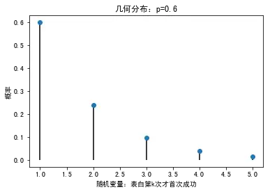
3 几何分布

*# 1 第k次做某件事情，才获得第一次成功*``k``**=**``5 p``**=**``0.6 X``**=**``np``**.**``arange(1,k``**+**``1,1) X array([1, 2, 3, 4, 5]) ``*# 2 求概率*``pList``**=**``stats``**.**``geom``**.**``pmf(X,p) pList array([ 0.6 , 0.24 , 0.096 , 0.0384 , 0.01536]) ``*# 3 绘图*``plt``**.**``plot(X,pList,marker``**=**``'o',linestyle``**=**``'None') plt``**.**``vlines(X,0,pList) plt``**.**``xlabel('随机变量：表白第k次才首次成功') plt``**.**``ylabel('概率') plt``**.**``title('几何分布：p=0.6') plt``**.**``show()

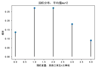
4 泊松分布

*# 1 定义随机变量*``*# 发生事故的比率是2次，一天发生k次事故的概率是多少*``mu``**=**``2 ``*#均值*``k``**=**``4 ``*#第四次发生的概率*``X``**=**``np``**.**``arange(0,k``**+**``1,1) X array([0, 1, 2, 3, 4]) ``*# 2 求概率*``pList``**=**``stats``**.**``poisson``**.**``pmf(X,mu) pList array([ 0.13533528, 0.27067057, 0.27067057, 0.18044704, 0.09022352]) ``*# 3 绘图*``plt``**.**``plot(X,pList,marker``**=**``'o',linestyle``**=**``'None') plt``**.**``vlines(X,0,pList) plt``**.**``xlabel('随机变量：某路口发生k次事故') plt``**.**``ylabel('概率') plt``**.**``title('泊松分布：平均值mu=2') plt``**.**``show()

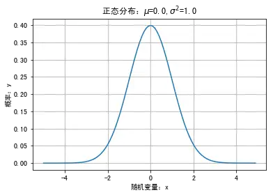
5 正态分布

*# 1 定义随机变量*``mu``**=**``0 sigma``**=**``1 ``*#标准差*``X``**=**``np``**.**``arange(``**-**``5,5,0.1) X array([ ``**-**``5.00000000e+00, ``**-**``4.90000000e+00, ``**-**``4.80000000e+00, ``**-**``4.70000000e+00, ``**-**``4.60000000e+00, ``**-**``4.50000000e+00, ``**-**``4.40000000e+00, ``**-**``4.30000000e+00, ``**-**``4.20000000e+00, ``**-**``4.10000000e+00, ``**-**``4.00000000e+00, ``**-**``3.90000000e+00, ``**-**``3.80000000e+00, ``**-**``3.70000000e+00, ``**-**``3.60000000e+00, ``**-**``3.50000000e+00, ``**-**``3.40000000e+00, ``**-**``3.30000000e+00, ``**-**``3.20000000e+00, ``**-**``3.10000000e+00, ``**-**``3.00000000e+00, ``**-**``2.90000000e+00, ``**-**``2.80000000e+00, ``**-**``2.70000000e+00, ``**-**``2.60000000e+00, ``**-**``2.50000000e+00, ``**-**``2.40000000e+00, ``**-**``2.30000000e+00, ``**-**``2.20000000e+00, ``**-**``2.10000000e+00, ``**-**``2.00000000e+00, ``**-**``1.90000000e+00, ``**-**``1.80000000e+00, ``**-**``1.70000000e+00, ``**-**``1.60000000e+00, ``**-**``1.50000000e+00, ``**-**``1.40000000e+00, ``**-**``1.30000000e+00, ``**-**``1.20000000e+00, ``**-**``1.10000000e+00, ``**-**``1.00000000e+00, ``**-**``9.00000000e-01, ``**-**``8.00000000e-01, ``**-**``7.00000000e-01, ``**-**``6.00000000e-01, ``**-**``5.00000000e-01, ``**-**``4.00000000e-01, ``**-**``3.00000000e-01, ``**-**``2.00000000e-01, ``**-**``1.00000000e-01, ``**-**``1.77635684e-14, 1.00000000e-01, 2.00000000e-01, 3.00000000e-01, 4.00000000e-01, 5.00000000e-01, 6.00000000e-01, 7.00000000e-01, 8.00000000e-01, 9.00000000e-01, 1.00000000e+00, 1.10000000e+00, 1.20000000e+00, 1.30000000e+00, 1.40000000e+00, 1.50000000e+00, 1.60000000e+00, 1.70000000e+00, 1.80000000e+00, 1.90000000e+00, 2.00000000e+00, 2.10000000e+00, 2.20000000e+00, 2.30000000e+00, 2.40000000e+00, 2.50000000e+00, 2.60000000e+00, 2.70000000e+00, 2.80000000e+00, 2.90000000e+00, 3.00000000e+00, 3.10000000e+00, 3.20000000e+00, 3.30000000e+00, 3.40000000e+00, 3.50000000e+00, 3.60000000e+00, 3.70000000e+00, 3.80000000e+00, 3.90000000e+00, 4.00000000e+00, 4.10000000e+00, 4.20000000e+00, 4.30000000e+00, 4.40000000e+00, 4.50000000e+00, 4.60000000e+00, 4.70000000e+00, 4.80000000e+00, 4.90000000e+00]) ``*# 2 求概率：概率密度函数 PDF*``y``**=**``stats``**.**``norm``**.**``pdf(X,mu,sigma) ``*# 3 绘图*``plt``**.**``plot(X,y) plt``**.**``xlabel('随机变量：x') plt``**.**``ylabel('概率：y') plt``**.**``title('正态分布：$\mu$=%.1f,$\sigma^2$=%.1f'``**%**``(mu,sigma)) plt``**.**``grid() plt``**.**``show()